Line charts & sampling time series data sets

When venturing in dataviz space one quickly runs into the task of visualizing a time series dataset. There are ample examples to be collected just about everywhere. The obvious chart type to visualize such a data set is a line chart.

One of the factors to take into account when moving from the raw time series data to its line chart representation is that oftentimes the resolution of the data set is higher than what makes sense for the medium one wants to display the chart on. Trying to plot thousands of data points on a screen of a few hundred pixels wide (think mobile device) does not make sense. One risks ending up with a visual mess while at the same time transferring and rendering all the data points will waste bandwidth and processing resources.

Two types of solutions are commonly applied to avoid the above-mentioned pitfalls. One can either aggregate groups of adjacent data points (e.g take the average of a hundred consecutive values) or alternative subsample the data set (e.g. keep one data point out of every hundred). In both cases, one ends up with substantially fewer data points at the cost of losing information. Depending on what aspect of the data set one wants to highlight one approach is more suited than the other.

An SQL implementation of the ‘Largest Triangle Three Bucket’ algorithm

In what follows, a SQL implementation of the ‘Largest Triangle Three Bucket’ (LTTB) sampling algorithm is discussed. This algorithm, as explained in detail in the master thesis of Sveinn Steinarsson, has the interesting characteristic that even after a substantial data set size reduction, the overall graph contour is represented fairly accurately. For the motivation behind the design choices of this algorithm refer to the thesis mentioned.

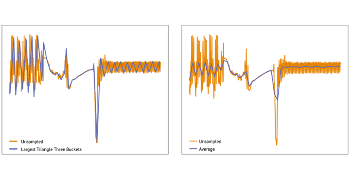
An example of the algorithm’s effect can be seen in the figure below. For comparison, also the result of the above-mentioned average aggregation is shown. As can be observed, the sampling algorithm manages to follow the contours of the unsampled data set better than the average aggregation does. In this example, the sampled (or aggregated) data set contains 50 data points while the unsampled data set contains 850 data points. Depending on what aspect of the data the graph needs to highlight, one or the other data reduction approach should be considered.

A step by step overview of the LTTB algorithm

• To start, the data set is divided into buckets. The number of buckets will determine the size of the data set after sampling.
• The first bucket contains only one data point, namely the first.
• The last bucket contains only one data point, namely the last.
• All other data points are divided over the other buckets.
• The algorithm will select for each of the buckets one data point such that the surface of the triangle formed by the data point selected from the ‘previous’ bucket, the data point selected from the ‘current’ bucket, and the data point selected from the ‘following’ bucket is maximized.
• Because the first bucket contains only one data point and the algorithm moves from ‘left to right’, determining the selected data point of the ‘previous’ bucket is easy. When working on the second bucket, it’s the only data point of the first bucket. For the nth bucket, it’s the data point selected in the previous step of the algorithm.
• The question is which data point to select from the ‘following’ bucket. Ideally, all data points of the ‘following’ bucket should be considered, but in order to reduce the search space (and execution time), the algorithm calculates the average of the data points in the ‘following’ bucket and uses that to determine the data point to select for the ‘current’ bucket. This average data point is ignored as soon as the algorithm moves on to the next bucket.

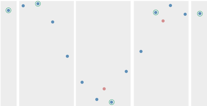
The different aspects of the LTTB algorithm are displayed in the figure below. The blue dots represent the original data, grey bands show the buckets, the orange dots are the ‘average’ values for the buckets and the green circled blue dots are the LTTB sampled data points.

How to implement the LTTB algorithm in SQL

While the LTTB algorithm is not difficult to implement in a general-purpose programming language, it’s not obvious to implement in SQL. Nevertheless, time series data is oftentimes stored in a relational database. As such it makes sense to subsample at the level of the database. This will limit the amount of data to be selected and transferred from the database server to the visualization environment.

The SQL implementation discussed in what follows is based on PostgreSQL (9.6), but it should be possible to convert to other SQL implementations that support user-defined aggregate functions and recursive common table expressions (CTE).

The first two data types are created.

Also, a helper function to calculate the surface of the triangle formed by its three input arguments will be useful in what follows.

Then a user-defined aggregate function is created, ‘largest_triangle’. The details of how to create PostgreSQL user-defined aggregate functions are explained in many other places and are beyond the scope of the current discussion.

The SQL to create this aggregate function (and its accompanying accumulator) follows.

Given a set of three data points, the aggregate function will return one of those data points and the surface of the triangle formed by these three data points such that the surface is the maximum for the input data set.

A simple example

At this point, the SQL implementing the LTTB algorithm can be introduced. Before attempting to understand the code, it’s important to be familiar with SQL’s recursive common table expressions (CTE) and window functions. Ample information is available elsewhere, including the official PostgreSQL documentation.

The SQL starts from a simple table with two columns: timestamp and value. The final result is a result set with the same structure but with only a fraction of the rows. How big a fraction is determined by a parameter, ‘bucketsize’ that is introduced in a first ‘dummy’ CTE. Such a dummy CTE is a convenient way to have the input values only in one place in the SQL.

The 3600 indicates that buckets will span 1 hour so that the algorithm will keep one data point per hour.

Then follows a query that returns the time series data set that has to be sampled. As long as this query returns a result set with a timestamp and value column the rest of the LTTB SQL will work without modifications. This query will typically filter rows from a large time series table using some application-specific set of tables, join and filter criteria: e.g. start and stop timestamps, device name, …

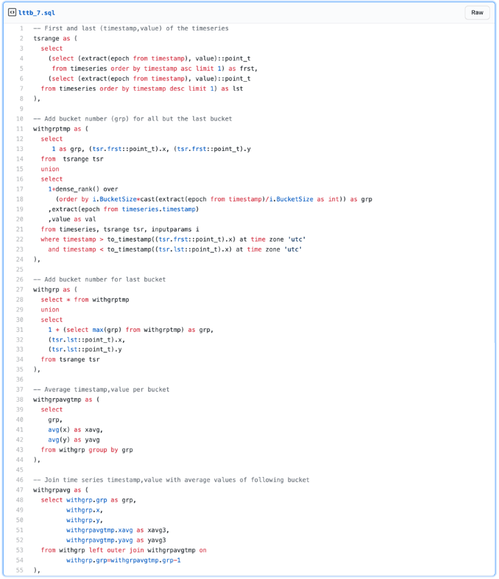
Next follows a sequence of CTE’s that add the bucket number to the ‘timestamp,value’ tuple and the ‘average’ timestamp and ‘average’ value of the ‘following’ bucket. Because the first and last bucket should contain the first and last data point of the time series, there is some extra processing needed to handle those properly.

At this point the ‘witgrpavg’ CTE returns a result set like:

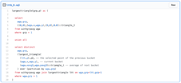
The last CTE is the trickiest one. It needs to select a ‘timestamp,value’ per bucket such that the surface of the triangle formed by the selected ‘timestamp,value’ of the previous bucket, the current ‘timestamp,value’ and the average values of the next bucket is maximized. The difficulty is where to get the selected ‘timestamp,value’ from the previous bucket. As explained higher, conceptually that is not difficult, but expressing it in SQL is less trivial. It requires a recursive CTE like so:

Notes:

• The first select of this CTE covers the first bucket case (grp=1).
• Because the largest_triangle function returns a ‘triange_t’ result some dummy values need to be added to this first select. The only relevant part of this ‘triangle_t’ value will be ‘p2’ anyway as will become clear later.
• The second select ‘recursively’ queries the result set that is being created to find the ‘triangle_t’ for the previous bucket (wga.grp=ltt.grp+1) and uses that ( (ltt.p).p2 ) to invoke the largest_triangle aggregate function with the current ‘timestamp,value’ (wga.x,wga.y) and average ‘timestamp,value’ of the next bucket (wga.xavg3,wga.yavg3).

Finally, the ‘largesttriangle’ result set created by this recursive CTE, is queried to return the LTTB sampled ‘timestamp,value’ values per bucket.

A complete demo gist is available. To make it work on real data you will want to change two parts: the value for BucketSize and the query that returns the time series data.